Graphical Interface

This part discusses the use of the Graphical User Interface (GUI). For tutorial on using tesliper in Python scripts, see tutorial.

On Windows system you may start the GUI by downloading and double-clicking Tesliper.exe file available in the latest release, as described in the Installation section. Executable files are not available for other systems, unfortunately, but you may start the GUI from the command line as well:

$ python -m pip install tesliper[gui]  # only once
$ tesliper-gui  # starts GUI

Note

If you’d like to start the graphical interface from the local copy, you may also run it as a module with python -m tesliper.gui.

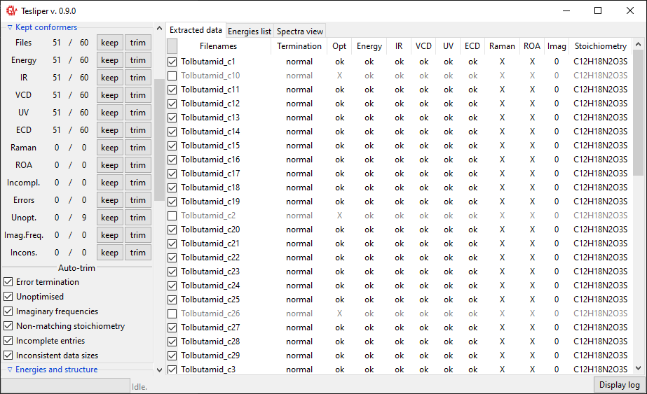
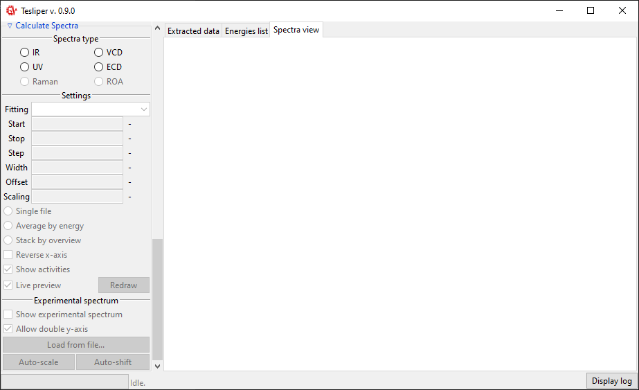
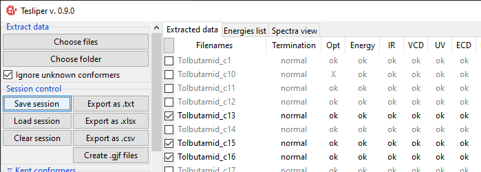
Please note that the first launch may take additional time. After the application starts, a window like the one bellow will appear. It’s actual looks will depend on your operating system.

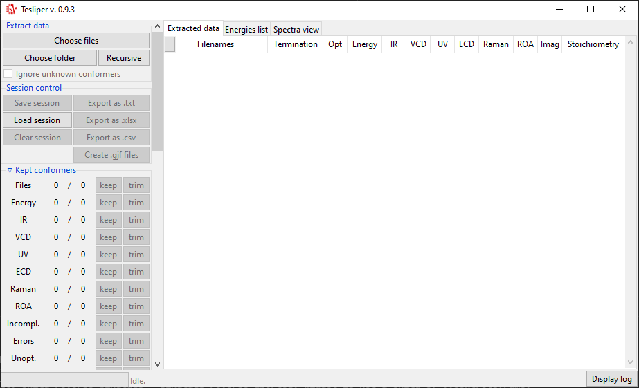
The Interface is divided in two parts: controls on the left and views (initially empty) on the right. Controls panel are further divided into sections, some of which may be collapsed by clicking on the section title (those with a small arrow on the left). Each section will be described further in this tutorial, in the appropriate section.

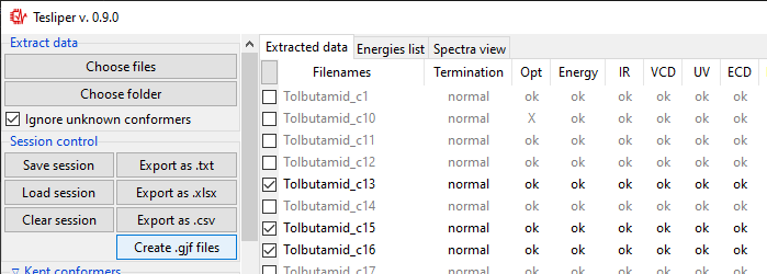
There are tree views available: Extracted data and Energies list summarize all conformers read from files. Extracted data details what data is available and shows status of calculations for each conformer. Energies list shows values of conformers’ energies calculated by quantum chemical software and derived values: Boltzmann factors and conformers’ populations.

Reading files

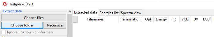
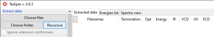
tesliper supports reading data from computations performed using Gaussian software. To load data, use controls in the Extract data section. Choose files button allows you to select individual files to read using the popup dialog. Choose folder button shows a similar dialog, but allowing you to select a single directory - all Gaussian output files in this directory (but not subdirectories) will be read. Finally, using the Recursive button will also read files form all subdirectories, recursively.

Note

Make sure you do not have mixed .log and .out files in the directory, when using Choose folder button.

Once you select files or directory and confirm your selection, the process of data extraction will start and Extract data view will be updated for each read conformer. It will show if calculation job terminated normally (Termination), if conformer’s structure was optimized and if optimization was successful (Opt), if extended set of energies is available (Energy), what spectral data it available (IR, VCD, UV, ECD, Raman, ROA), how many imaginary frequencies are reported for conformer (Imag), and what is conformer’s stoichiometry (Stoichiometry).

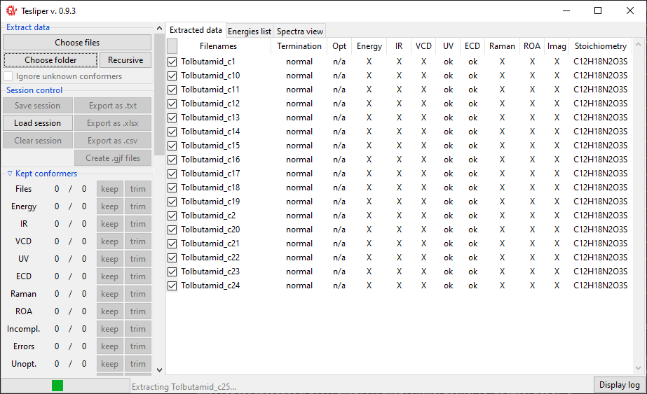
When data extraction is finished, the status barr att the bottom will show Idle again. After reading first portion of files, you may tick the Ignore unknown conformers option. When this option is ticked, tesliper will only read files that correspond to conformers it already knows (judging by the filename).

Trimming conformers

Conformers may be marked as kept not kept (trimmed). Only kept conformers are processed by tesliper, trimmed ones are ignored. This mechanism allows you to select which conformers should be included in the final averaged spectrum, etc. Trimmed conformers are shown in gray.

Kept conformers section shows how many conformers contain certain data and allows to easily keep/trim whole groups of conformers, using keep and trim buttons beside the appropriate group. You may also keep/trim individual conformers by ticking/unticking checkboxes beside the conformers name (left of Filenames column).

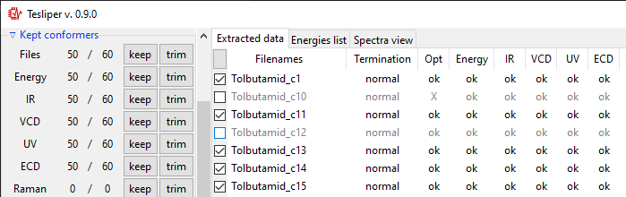
After finished data extraction and after each manual trimming, auto-trimming is performed to make sure corrupted or invalid conformers are not accidentally kept. Checkboxes in the Auto-trim subsection, shown below, control which conformers should be always trimmed.

Tip

Incomplete entries are conformers that miss some data, which other conformers include, e.g. those that were left out in one of calculations steps. Inconsistent data sizes indicates that some multi-value data has different number of data points than in case of other conformers. This usually suggests that conformer in question is not actually a conformer but a different molecule.

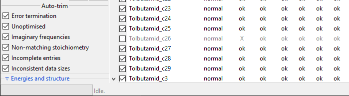
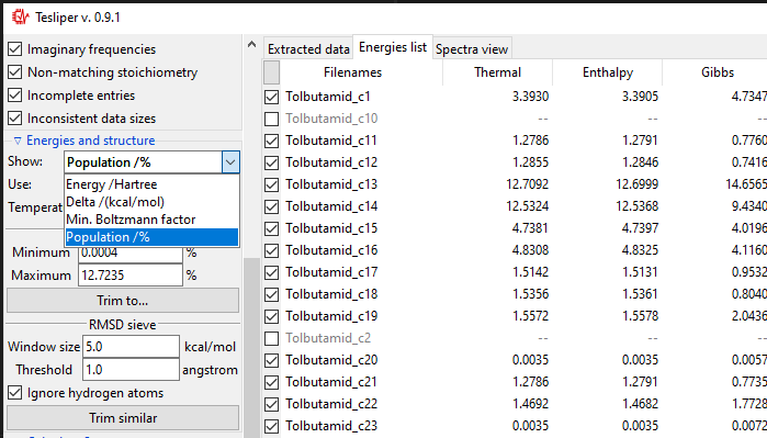
Trimming with sieves

The Energies and structure section, described in this part, is related with the Energies list view. This view shows, as the name suggests, list of energies for each conformer and energies-derived values.

Using a Show: drop-down menu you may select a different energies-derived data to show in the view. Delta is conformer’s energy difference to the most stable (lowest-energy) conformer (in \(\mathrm{kcal}/\mathrm{mol}\) units), Min. Boltzmann factor is conformer’s Boltzmann factor in respect to the most stable conformer (unitless) and Popuation is population of conformers according to the Boltzmann distribution (in perecnt). Original Energy values are shown in Hartree units.

Both types of sieves provided depend on the selected value of the Use: drop-down menu. It determines, which energy values are used by the sieves. Only available energies wil be shown in the list. In case their names are not intuitive enough, here is the explanation:

Thermal: sum of electronic and thermal Energies;

Enthalpy: sum of electronic and thermal Enthalpies;

Gibbs: sum of electronic and thermal Free Energies;

SCF: energy calculated with the self-consistent field method;

Zero-Point: sum of electronic and zero-point Energies.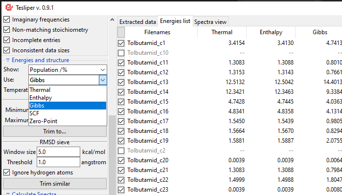

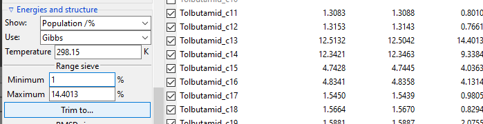
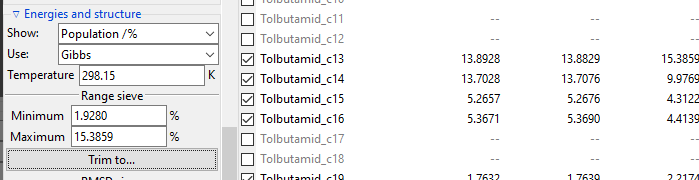
The Range sieve lets you to trim conformers that have a current Show: value outside of the specified range. After you fill the Minimum and Maximum fields to match your needs, click Trim to... button to perform trimming. The example below shows trimming of conformers, which Free Energy-derived population is below 1%. Please note that valuesin the Energies list are recalculated and Minimum and Maximum fields are updated to show real current max and min values.

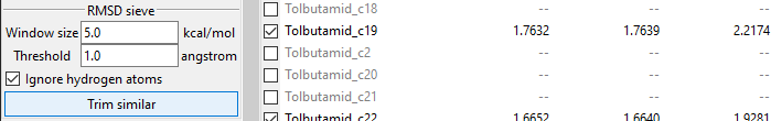
The RMSD Sieve lets you mathematically compare structures of conformers and trim duplicates and almost-duplicates. RMSD stands for root-mean-square deviation of atomic positions and is a conformers similarity measure. The sieve calculates the average distance between atoms of two conformers and trims the less stable (higher-energy) conformer of the two, if the resulting RMSD value is smaller than value ot the Threshold field.

Calculating an RMSD value is quite resource-costly. To assure efficient trimming, each conformer is compared only with conformers inside its energy window, defied by the Window size filed value. Conformers of energy this much higher or lower are automatically considered different.

Temperature of the system

The Energies and structure section also allows you to specify the temperature of the studied system. This parameter is important for calculation of the Boltzmann distribution of conformers, which is used to estimate conformers’ population and average conformers’ spectra. The default value is the room temperature, expressed as \(298.15\ \mathrm{Kelvin}\) (\(25.0^{\circ}\mathrm{C}\)). Changing this value will trigger automatic recalculation of Min. Boltzmann factor and Population values, and average spectra will be redrawn.

New in version 0.9.1: The Temperature entry allowing to change the temperature value.

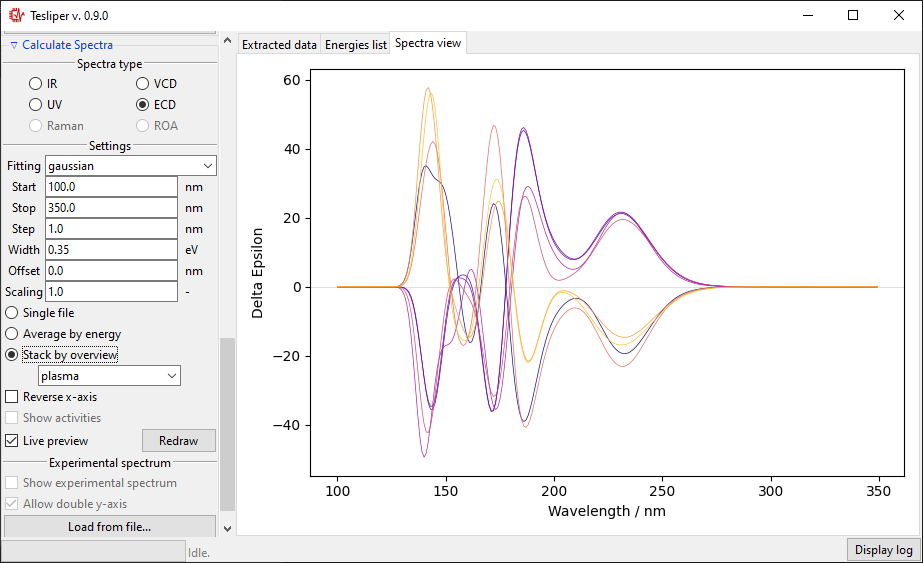
Spectra simulation

Calculate Spectra controls section and Spectra view tab allow to preview the simulation of selected spectrum type with given parameters.

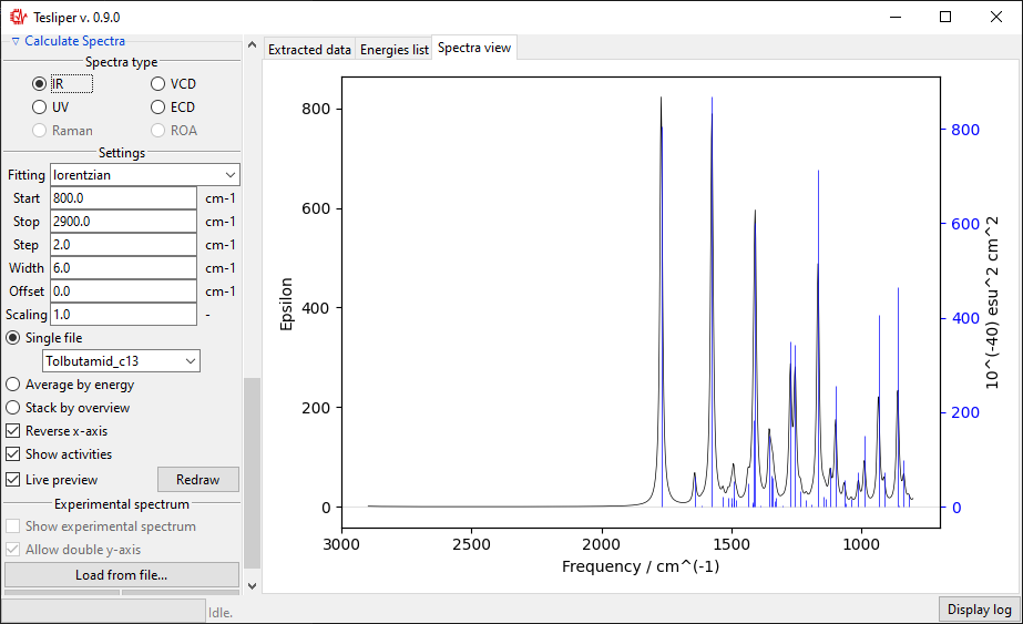
The Spectra view tab is initially empty, but when you select one of the available Spectra types, Settings subsection will become enabled and the spectrum will be drawn.

Tip

You can turn off automatic recalculation of the spectrum by unchecking the Live preview box.

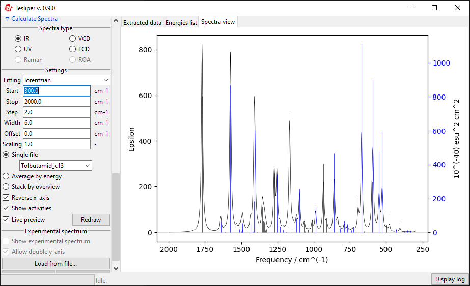
Beginning and end of the simulated spectral range may be set using Start and Stop fields. The view on the right will match these boundaries. Please note that Start must have lower value than Stop. There is also a Step field that allows you to adjust points density in the simulated spectrum.

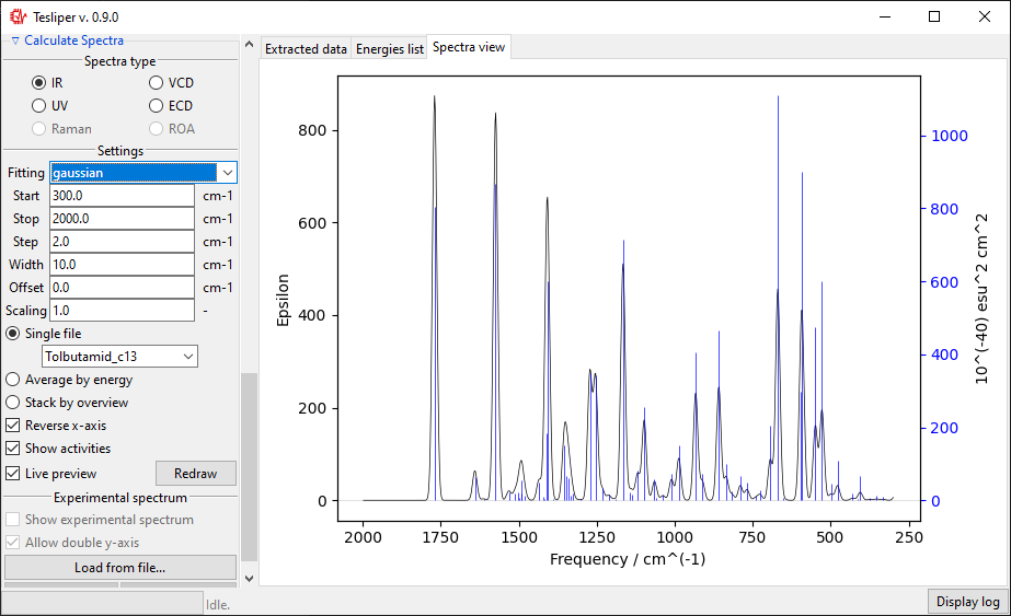
Width field defines a peak width in the simulated spectrum. It exact meaning depends on the chosen fitting function (see below). For gaussian fitting Width is interpreted as half width of the peak at \(\frac{1}{e}\) of its maximum value (HW1OeM). For lorentzian function it is interpreted as half width at half maximum height of the peak (HWHM).

Tip

You may change fields’ values with the mouse wheel. Point the field with mouse cursor and allow for a small delay before switching form the scroll mode to the value-changing mode. Move the mouse cursor away from the field to switch back.

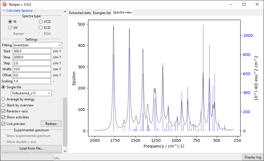
Finally, you may choose the fitting function used to simulate the spectrum from the calculated intensities values - this will have a big impact on simulated peaks’ shape. Two such functions are available: gaussian and lorentzian functions. Usually lorentzian function is used to simulate vibrational spectra and gaussian function for electronic spectra.

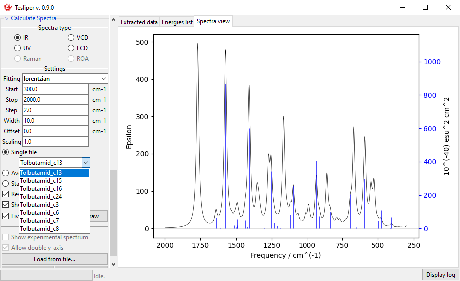
The default spectra preview is a Single file preview that allows you to see the simulated spectrum for the selected conformer. You may change the conformer to preview using the drop-down menu shown in the screenshot below.

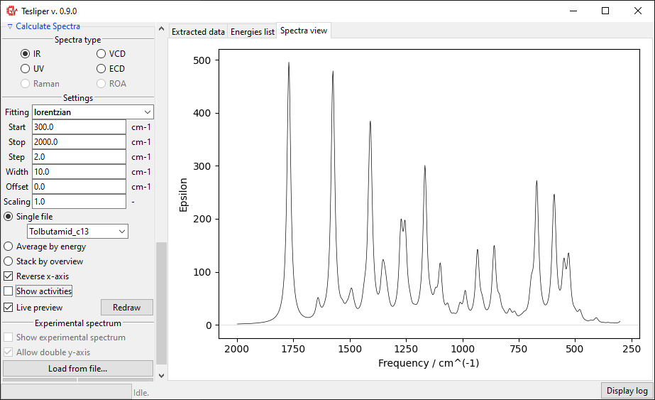
When in a Single file preview, spectral activities used to simulate the spectrum are also shown on the right. You may turn this off by unticking the Show activities box.

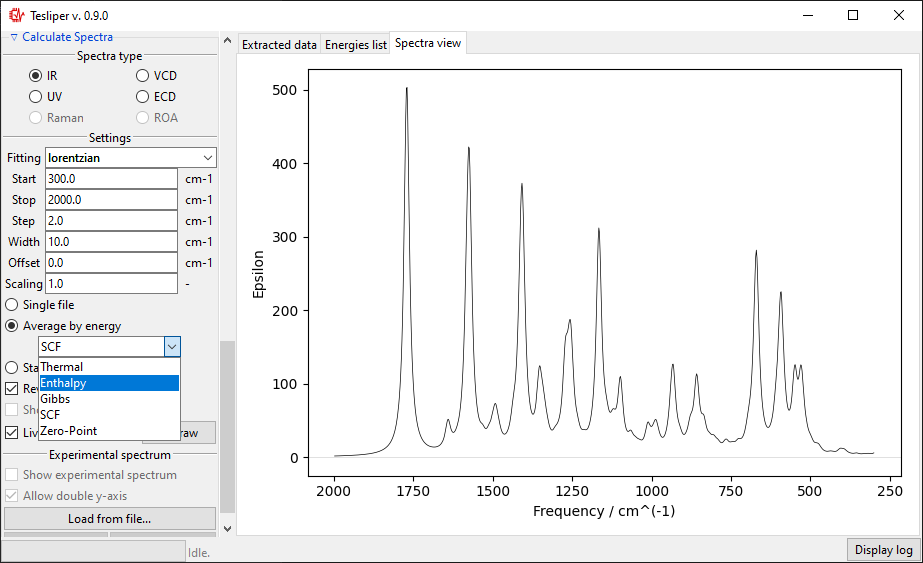
You can also preview an population-weighted average spectrum of all kept conformers, by selecting Average by energy. The drop-down menu lets you select the energies that tesliper should use to calculate conformers populations.

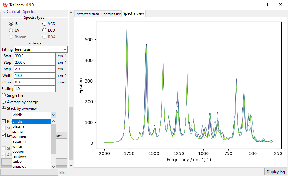
The final option is to show all kept conformers at once by selecting Stack by overview option. The drop-down menu allows to choose a color scheme for the stacked spectra lines.

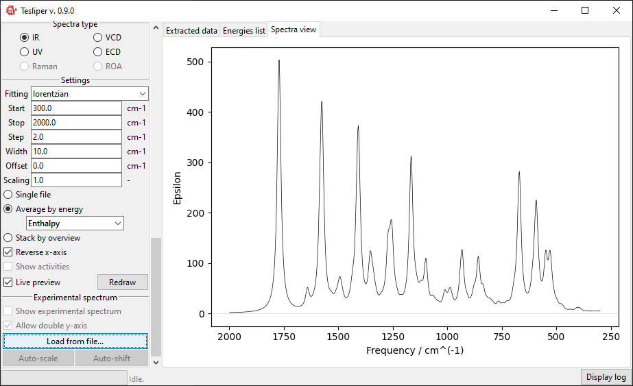
Comparing with experiment

It’s possible to and an overlay with the experimental spectrum to Single file and Average by energy previews. To load an experimental spectrum, use Load from file button in the Experimental spectrum subsection. tesliper can read spectrum in the .txt (or .xy) file format. Binary .spc formats are not supported.

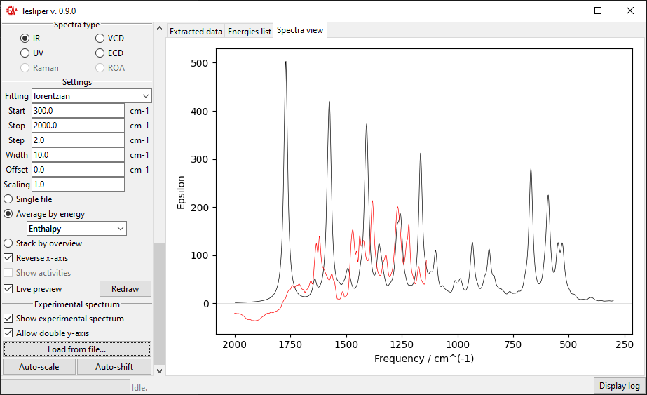
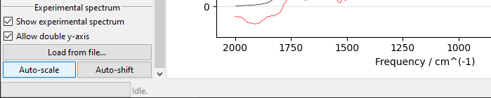
When you choose the experimental spectrum file, it’s curve is drown on the right with respect to the Start and Stop bounds. Red color is used for the experiment. In case of a significant difference in the magnitude of intensity in both spectra, the second scale will be added to the drawing.

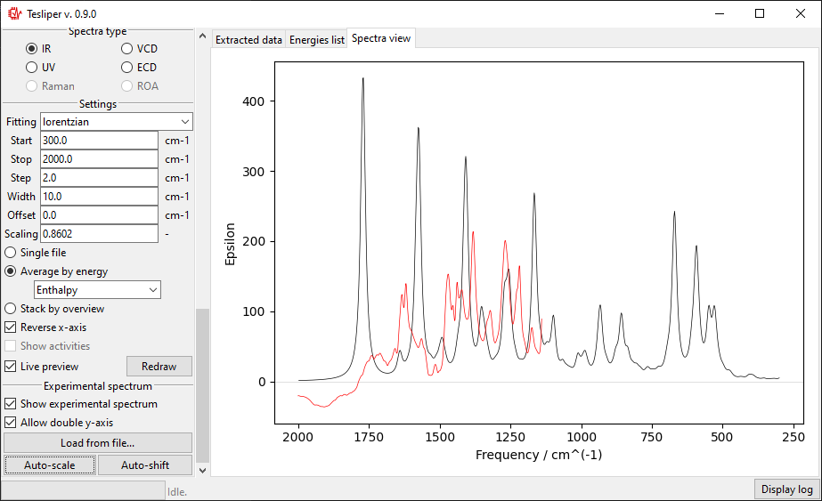
The scale of the simulated values may be automatically adjusted to roughly match the experiment with the Auto-scale button. It may be also adjusted manually by changing the value of the Scaling field.

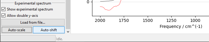
Similarly, Auto-shift button and Offset field let you to adjust simulated spectrum’s position on the x-axis. Positive Offset shifts the spectrum bathochromically, a negative one shifts it hypsochromically.

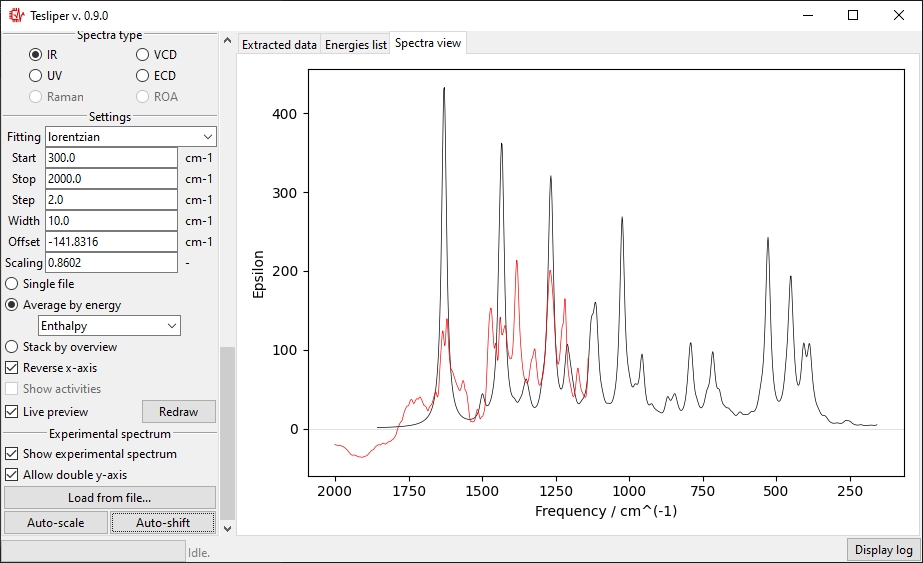
Scaling and Offset values are remembered for the current spectra type, just like the other parameters.

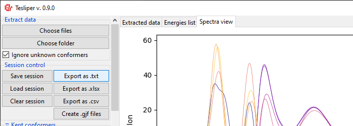
Data export

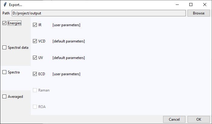
Calculated and extracted data may be exported to disk in three different formats: text files with Export to .txt button, csv files with Export to .csv button and Excel files with Export to .xlsx button. Clicking on any of those will bring up the Export... dialog.

At the top of the Export... dialog is displayed the path to the currently selected output directory. It may be changed by clicking on the Browse button and selecting a new destination. Files generated by tesliper will be written to this directory.

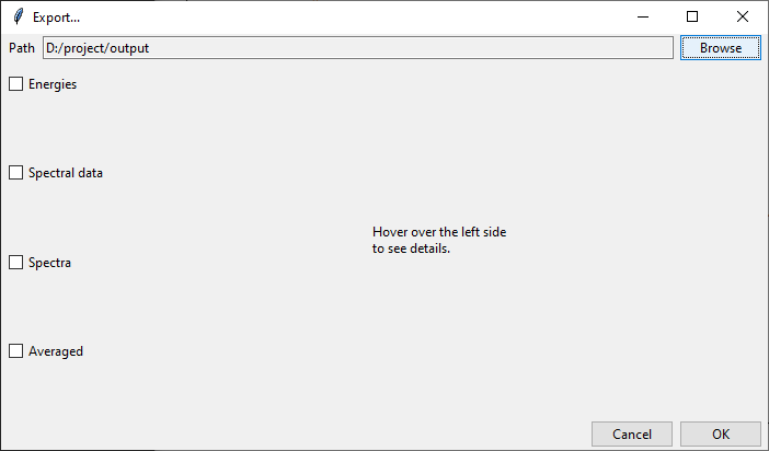
On the left side of the dialog window you may select what type of data you want to export by ticking appropriate boxes. Once you hover over the certain category, more detailed list of available data will be shown on the right. By ticking/unticking selected boxes you can fine-tune what should be written to disk.

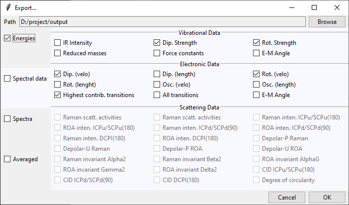
In the Spectra category, beside each available spectra type, there is a note that informs if calculation parameters were altered by the user. Spectra will be recalculated with current parameters upon the export confirmation.

Creating Gaussian input

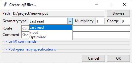
Clicking on the Create .gjf files... will open a dialog window that lets you setup a next step of calculations to conduct with the Gaussian software.

Similarly to the previews one, this dialog also features a Path field that specifies the output directory, which may be changed by clicking on the Browse button. Bellow it is the Geometry type drop-down menu that allows you to select, which geometry specification should be used in the new input files. Input is the geometry used as an input in the extracted .log/.out files, Last read is the one that was lastly encountered in these files. Optimized is the geometry marked as optimized by Gaussian, but it is only available from the successful optimization calculations. You also need to specify the Charge and the Multiplicity of the molecule.

Below are the Route and Comment fields. The first one specifies the calculation directives for the Gaussian software. The second one is a title section required by GAussian.

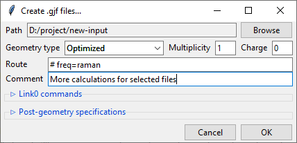
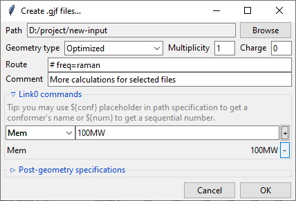
Further below is the expandable Link0 commands panel that allows to specify Link 0 directives, which define location of scratch files, memory usage, etc. Select a command name from the drop-down menu, filed on right will show a hint about its purpose.

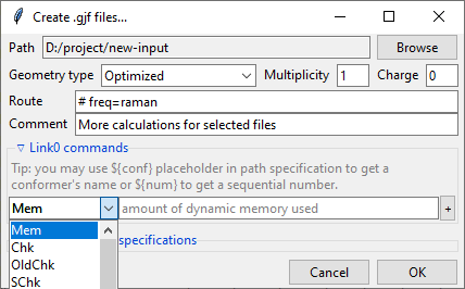
Provide a value in the input filed and click a + button to add a command. It will be added to the list below. You can update the selected command by providing a new value and clicking the + button again or remove it by clicking the - button.

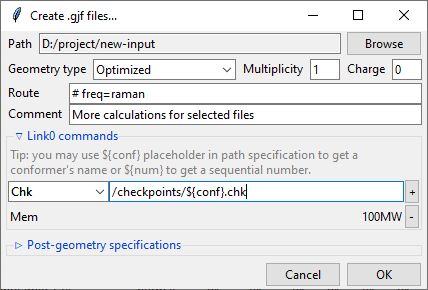
Path-like commands may be parametrized: ${conf} will be substituted with the name of conformer and ${num} will be substituted with the sequential number.

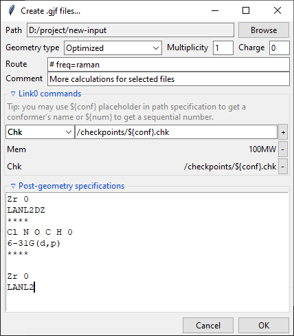
Finally, you can add a post-geometry specification. It will be written to the end of each .gjf file.

Saving session

You can save a session (all data, along with current trimmed and parameters) with a Save session button. A popup dialog will be opened, where you can specify a target session file location.

To load previously saved session use the Load session button. You can also discard all currently held data by clicking the Clear session button.

Warning

Loading and clearing session cannot be undone! A confirmation dialog will be displayed for those actions.